Image Mosaics With Python
02 January 2017

I'm sure you've seen an image mosaic before. Each pixel in the original image has been replaced with an entire image. The tiled, jagged result usually resembles the original image at a distance and, when good component images are chosen, presents the viewer with a very complex image to explore. Let's create some with python.
The General Idea
We start with a reference image: this is the image whose pixels will be replaced with individual tile images. The larger the image, the larger the output. I recommend you start small. Choose a relatively simple image, and scale it downwards. I've found that images in the size range of 20-30 pixels tall or wide produce good output.
The reference image should also not include transparency. When I was first writing this code, I couldn't figure out why the simple image I was using for a reference image never resulted in output that looked anything other than random. As I dug into the problem, I realized that every single pixel was the same color. But the image still looked like an image because each pixel had varied transparency. You can avoid this problem by ensuring your reference image is not transparent.
You can find the reference image for this article here.
This is what it looks scaled up to a visible size:

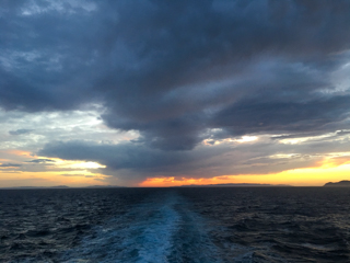
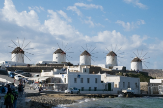
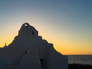
Yep. Cross of the Greek flag. I recently took a trip to Greece, and the pictures from the trip will also form our tile sources as well.
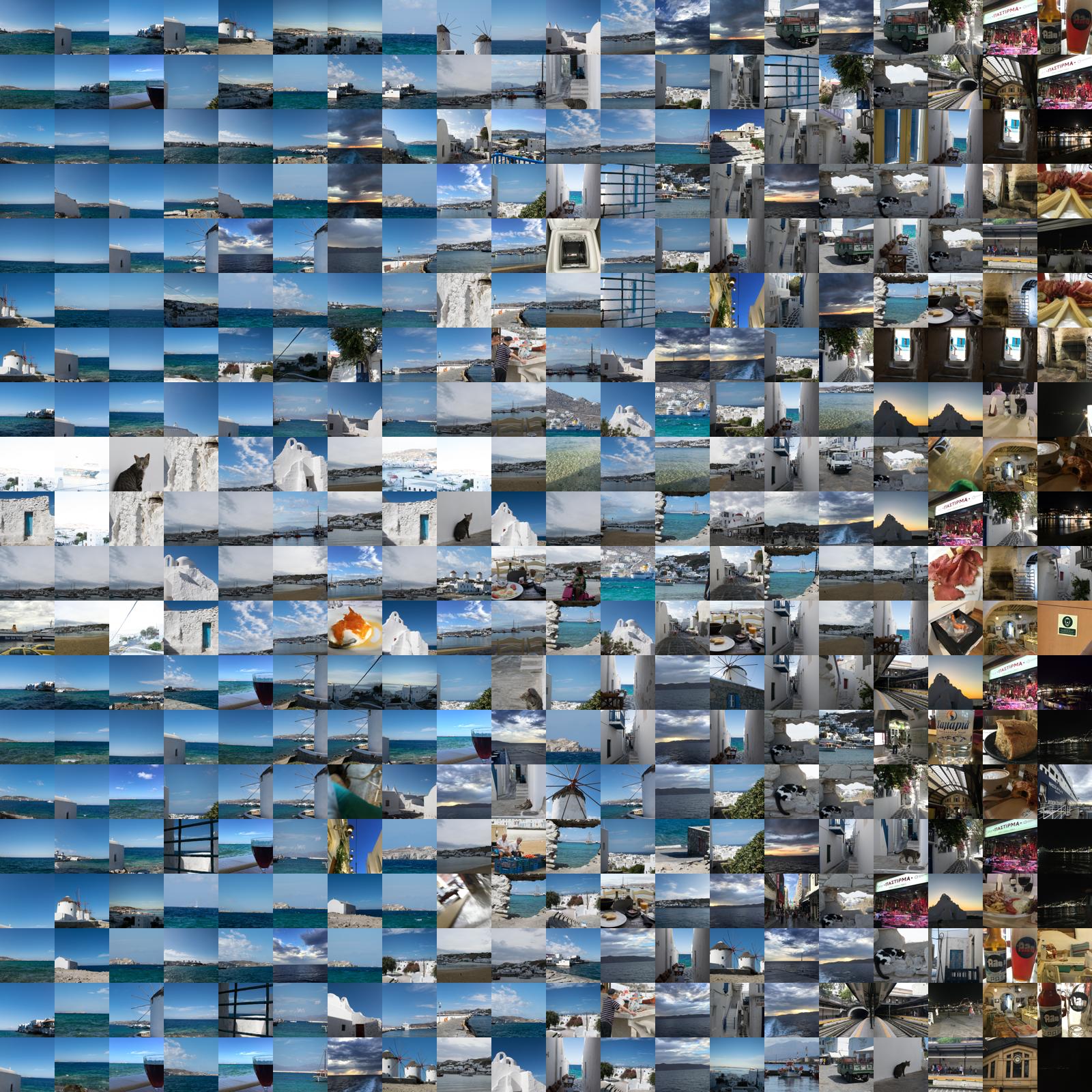
We also need a directory of images to use as sources. Each image will be cropped square and scaled down to the tile size as it is loaded. Technically, you can use other aspect ratios for the pixels of your mosaic. But the presented code doesn't allow for that. The images will be cropped square by trimming evenly from each side (i.e. a center-square crop). Other methods certainly exist: see my thumbify project for a look at alternative methods.
Each source image will then have its average color computed. The average color is computed by averaging the red, blue, and green channels individually and then returning that triple as the average color.
You can find the source images for this article here.
The last important idea is tile size. This is how large each component image of the mosaic is. The larger the tile size, the larger and more detailed the output image. However, there is a memory trade-off (in this implementation) with using larger tile sizes. I find a size of 80 works well from a memory and output size standpoint. You can then scale the final image as needed for printing, etc.
Our choice of libraries
Since I know next to nothing about how image processing
works in practice and because I'm way too lazy to even
explore reinventing this wheel, our image processing will
be done by pillow the PIL fork.
There's also some light math that I will handle by using
numpy (though, we could probably get on
without it).
If you're using the code from the repo (skip to the end for link), run the setup script. Otherwise just make sure you have these two dependencies installed. They're the only ones.
Loading our sources
As mentioned above, we load all of our source images up front and perform some preprocessing on them.
First, we crop the image:
def crop_image(img):

    if img.width > img.height:
        new_width = img.height
        new_height = img.height

        start_x = (img.width - img.height) / 2
        start_y = 0

        img = img.crop((
            start_x,
            start_y,
            start_x + new_width,
            start_y + new_height,
        ))
    elif img.height > img.width:
        new_width = img.width
        new_height = img.width

        start_x = 0
        start_y = (img.height - img.width) / 2

        img = img.crop((
            start_x,
            start_y,
            start_x + new_width,
            start_y + new_height,
        ))

    return img

source_image = crop_image(source_image)
Then we thumbnail the image to the appropriate tile size, to save on memory:
source_image.thumbnail((tile_size, tile_size))
Next, we'll convert the image to black and white (if
necessary) and force it to RGB. This step is necessary to
get r, g, b triples for calculating the
average color:
if not is_color:
    source_image = source_image.convert("L")

# always need to force into RGB only
source_image = source_image.convert("RGB")
And here we calculate the average color:
def average_color(img):
    """Return the average color of the given image.

    :param img: An image object.
    :returns: A three-tuple representing the average color.

    """

    h = img.histogram()

    # split into red, green, blue
    r = h[0:256]
    g = h[256:512]
    b = h[512:768]

    def wavg(s):
        """Find the weighted average of the sequence, which is a color channel.

        :param s: A color channel sequence.
        :returns: The weighted average.

        """

        # i is the index which is the channel value. w is the weight which is
        # the frequency of occurence.
        weighted = sum(i*w for i, w in enumerate(s))

        # sum of all values, which is how many times they occur
        total = sum(s)

        return int(weighted / float(total))

    return (wavg(r), wavg(g), wavg(b))

average_r, average_g, average_b = average_color(source_image)
You'll note that we're using the image's histogram to do this. You could also iterate of the image's pixels and compute the average that way, but the histogram method is faster. I had originally iterated over pixels, but the implementation was really too slow to be usable when the number of source images was large.
Here are some of our sample tile images converted to their average color:
| Before | After |
|---|---|
|

|
|

|
|

|
Varying shades of tinted gray. Alternatively, we could attempt to choose the most dominant color from the image. For images with a limited set of colors, this might be a better approximation of what the eye is seeing. Here are some examples of that:
| Before | After |
|---|---|
|
|

|
|
|

|
|
|

|
Some more intense color there, at least. The default is to
use average color, but commonest_color is
available as well.
Pixel selection
Now that our source images are loaded, we need to replace our pixels with images. Good mosaics limit repetition of images to the minimum amount possible. We'd like to mimic this, so we'll select from our pool of source images without replacement, until the pool is empty.
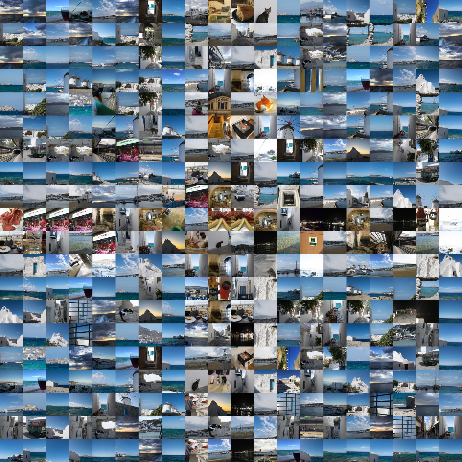
And yet, if we simply iterate over the pixels from left to right (or whatever simple pattern) as if we were reading the image left-to-right, the results will be less than optimal. All of the best matching images will cluster on the left, and the image will start to degrade in quality as we work our way across. Here's an example of what that looks like:
If we had a lot more source images, the problem wouldn't be as pronounced. Even with thousands of images, though, you can still run into this issue.
And the code:
def ordered_pixels(reference_image):

    pixels = []
    for x in range(reference_image.width):
        for y in range(reference_image.height):
            pixels.append((x, y))

    return pixels
The left-to-right pattern is a result of us iterating over columns, rather than rows. The pattern would just go top to bottom if we iterated y before x, though.
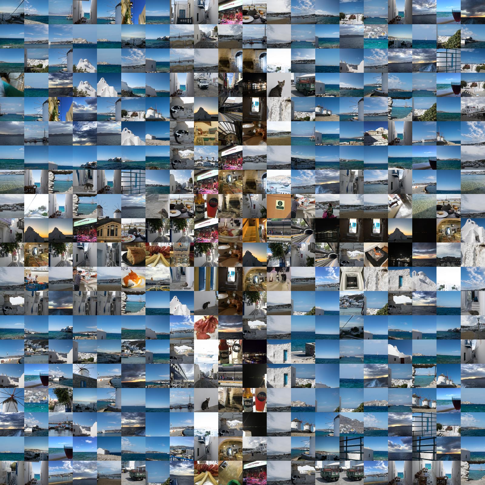
Moving on, we could attempt to improve on this by saying that midtones are the most important pixels and therefor should be filled first. Which is an improvement for our reference image:
Related code:
def midtone_pixels(reference_image):

    with_brightness = _pixels_with_brightness(reference_image)

    total_brightness = sum([b for b, _ in with_brightness])
    average_brightness = total_brightness / len(with_brightness)

    def midtone_sort(v):
        b, _ = v
        return abs(average_brightness - b)

    with_brightness.sort(key=midtone_sort)

    return [(x, y) for _, (x, y) in with_brightness]
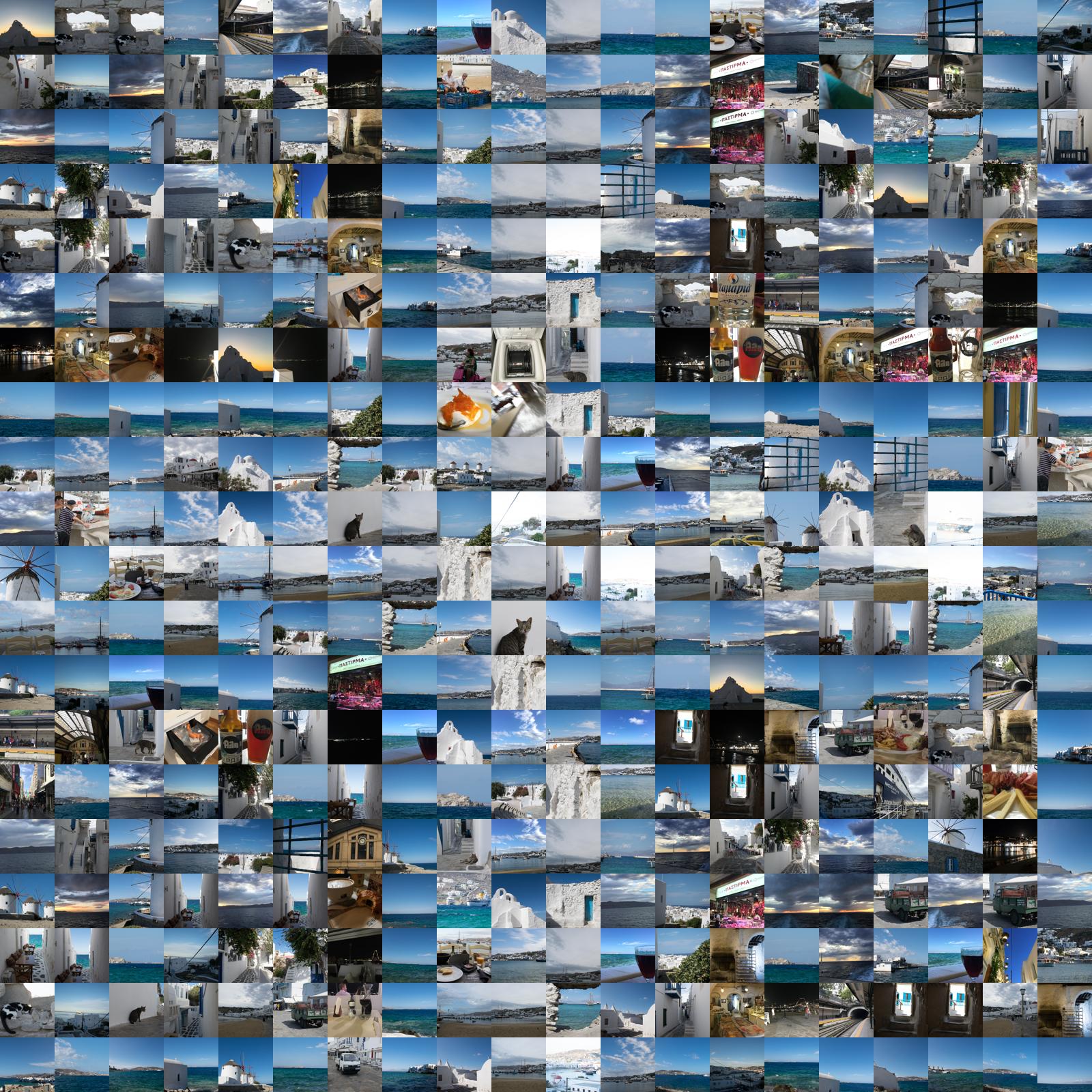
Darkest is an improvement, too:
Code for darkest:
def darkest_pixels(reference_image):

    with_brightness = _pixels_with_brightness(reference_image)

    with_brightness.sort()

    return [(x, y) for _, (x, y) in with_brightness]
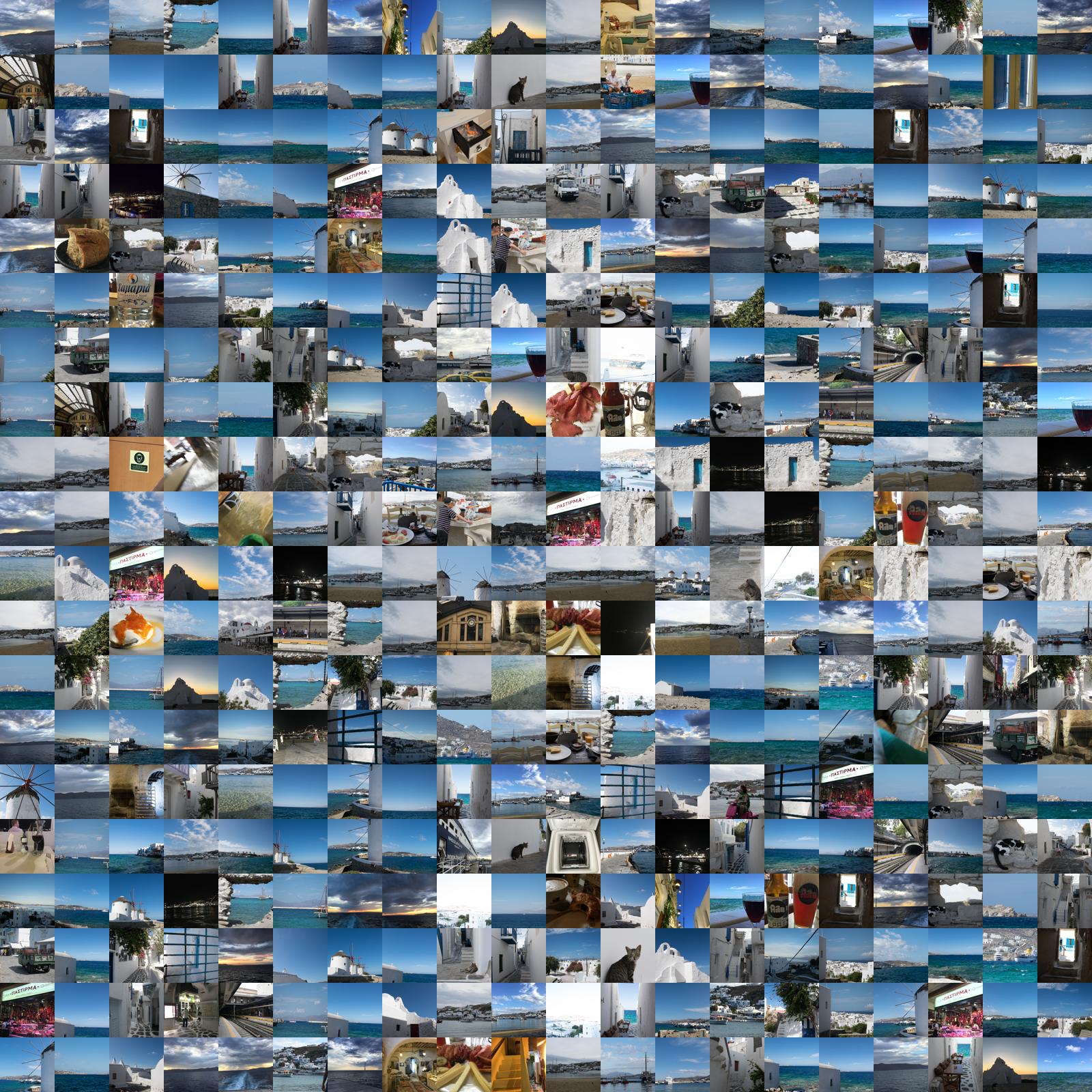
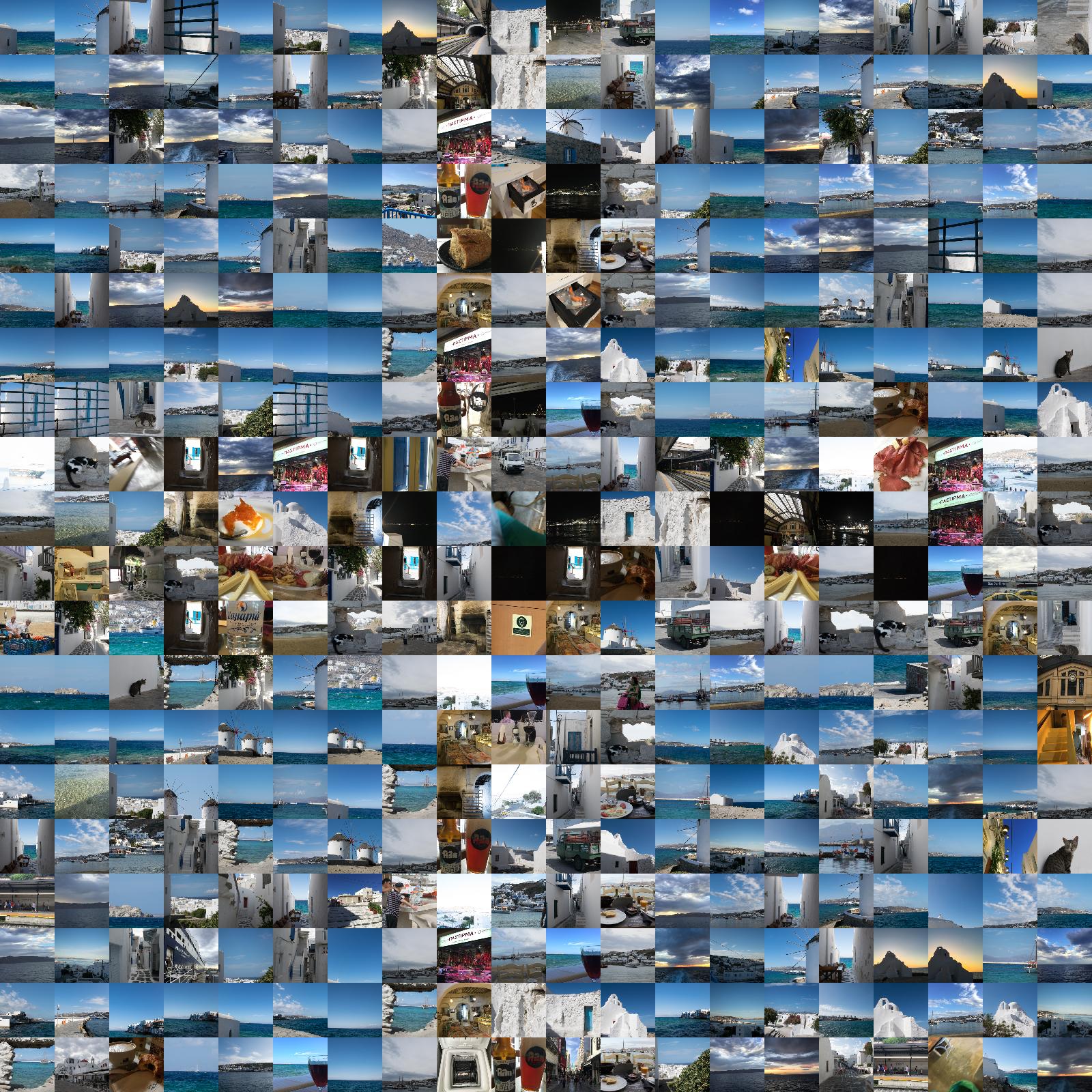
However, it seems brightest produces a good-er image for us:
And code for brightest:
def brightest_pixels(reference_image):

    pixels = darkest_pixels(reference_image)
    pixels.reverse()

    return pixels
I would say the output using darkest is probably slightly more defined, but the lightest is more true to the color of the original image.
Also note that if we had a different, more nuanced reference image and possibly a different set of source images, the outcome could be different. You may want to play around with these different methods to see if they offer an improvement for your purposes.
The default implementation is to choose pixels at random and try to fill them. You may not always get a great image on the first try, but run it a few times to generate a dozen or so candidates. You can then select the one that you think looks best. Which is, after all, important.
And the unintersting random code:
def random_pixels(reference_image):

    pixels = ordered_pixels(reference_image)

    random.shuffle(pixels)

    return pixels
Not an improvement over darkest. We'll choose darkest for our "final" image. Play around with the various options to see which produces a good output for you.
Finding matches
Once we've selected our pixels, we need to find a matching
image. We do this by comparing the "distance" between the
average color of the source images and the color of the
given pixel. We use the norm function from
numpy's linear algebra library to achieve
this. norm gives the length of a vector,
which we will use to determine how close each pixel and the
average color of each source image are:
pixel = reference_image.getpixel((x, y))
r = pixel[0]
g = pixel[1]
b = pixel[2]
reference_vec = numpy.array([[r, g, b]])

normed_images = []
for image, avg_color in pool:
    source_vec = numpy.array([avg_color])

    norm = numpy.linalg.norm(reference_vec - source_vec)
    normed_images.append((norm, image, avg_color))

normed_images.sort()
But we also don't want to be too greedy. If we always take the closest matching pixel, we tend to end up with similar images clustered in similar looking pixel locations. This isn't a very good look for the output.
Instead, we choose randomly among the closest 20:
top20 = normed_images[:20]
random.shuffle(top20)

_, selected_image, avg_color = top20[0]

pool.remove((selected_image, avg_color))
Other approaches
In researching this post, I came across a really cool article on the Wolfram blog about using Mathematica to create image mosaics. It goes through a bunch of other interesting approaches. I may cover the implementation of them in python in a future post.
Generating the ouptut
While we were selecting images for each pixel, we were
placing the source image of choice into an N x M matrix,
initially populated with Node.
After we've populated the matrix, we can simply walk over the rows and columns and paste each tile into the output image:
y_offset = 0
for row in output_matrix:

    x_offset = 0

    for image in row:

        paste_box = (
            x_offset,
            y_offset,
            x_offset + tile_size,
            y_offset + tile_size,
        )

        output_image.paste(image, paste_box)

        x_offset += tile_size

    y_offset += tile_size

return output_image
And that's it!
We also explored using the most common color above. Without revisiting every moscaic, let's see what a final ouptut using the most common color looks like:
Do you have this code somewhere that I can use it?
Funny you should ask! Yes: GitHub.